Optimization in R

Optimization is a very common problem in data analytics.  Given a set of variables (which one has control), how to pick the right value such that the benefit is maximized.  More formally, optimization is about determining a set of variables x1, x2, … that maximize or minimize an objective function f(x1, x2, …).

Unconstrained optimization

In an unconstraint case, the variable can be freely selected within its full range.

A typical solution is to compute the gradient vector of the objective function [∂f/∂x1, ∂f/∂x2, …] and set it to [0, 0, …].  Solve this equation and output the result x1, x2 … which will give the local maximum.

In R, this can be done by a numerical analysis method.

> f <- function(x){(x[1] - 5)^2 + (x[2] - 6)^2}
> initial_x <- c(10, 11)
> x_optimal <- optim(initial_x, f, method="CG")
> x_min <- x_optimal$par
> x_min
[1] 5 6

Equality constraint optimization

Moving onto the constrained case, lets say x1, x2 … are not independent and then have to related to each other in some particular way: g1(x1, x2, …) = 0,  g2(x1, x2, …) = 0.

The optimization problem can be expressed as …
Maximize objective function: f(x1, x2, …)
Subjected to equality constraints:

• g1(x1, x2, …) = 0
• g2(x1, x2, …) = 0

A typical solution is to turn the constraint optimization problem into an unconstrained optimization problem using Lagrange multipliers.

Define a new function F as follows ...
F(x1, x2, …, λ1, λ2, …) = f(x1, x2, …) + λ1.g1(x1, x2, …) + λ2.g2(x1, x2, …) + …

Then solve for ...
[∂F/∂x1, ∂F/∂x2, …, ∂F/∂λ1, ∂F/∂λ2, …] = [0, 0, ….]

Inequality constraint optimization

In this case, the constraint is inequality.  We cannot use the Lagrange multiplier technique because it requires equality constraint.  There is no general solution for arbitrary inequality constraints.

However, we can put some restriction in the form of constraint.  In the following, we study two models where constraint is restricted to be a linear function of the variables:
w1.x1 + w2.x2 + … >= 0

Linear Programming

Linear programming is a model where both the objective function and constraint function is restricted as linear combination of variables.  The Linear Programming problem can be defined as follows ...

Maximize objective function: f(x1, x2) = c1.x1 + c2.x2

Subjected to inequality constraints:

• a11.x1 + a12.x2 <= b1
• a21.x1 + a22.x2 <= b2
• a31.x1 + a32.x2 <= b3
• x1 >= 0, x2 >=0

As an illustrative example, lets walkthrough a portfolio investment problem.  In the example, we want to find an optimal way to allocate the proportion of asset in our investment portfolio.

• StockA gives 5% return on average
• StockB gives 4% return on average
• StockC gives 6% return on average

To set some constraints, lets say my investment in C must be less than sum of A, B.  Also, investment in A cannot be more than twice of B.  Finally, at least 10% of investment in each stock.

To formulate this problem:

Variable: x1 = % investment in A, x2 = % in B, x3 = % in C

Maximize expected return: f(x1, x2, x3) = x1*5% + x2*4% + x3*6%

Subjected to constraints:

• 10% < x1, x2, x3 < 100%
• x1 + x2 + x3 = 1
• x3 < x1 + x2
• x1 < 2 * x2

> library(lpSolve)
> library(lpSolveAPI)
> # Set the number of vars
> model <- make.lp(0, 3)
> # Define the object function: for Minimize, use -ve
> set.objfn(model, c(-0.05, -0.04, -0.06))
> # Add the constraints
> add.constraint(model, c(1, 1, 1), "=", 1)
> add.constraint(model, c(1, 1, -1), ">", 0)
> add.constraint(model, c(1, -2, 0), "<", 0)
> # Set the upper and lower bounds
> set.bounds(model, lower=c(0.1, 0.1, 0.1), upper=c(1, 1, 1))
> # Compute the optimized model
> solve(model)
[1] 0
> # Get the value of the optimized parameters
> get.variables(model)
[1] 0.3333333 0.1666667 0.5000000
> # Get the value of the objective function
> get.objective(model)
[1] -0.05333333
> # Get the value of the constraint
> get.constraints(model)
[1] 1 0 0

Quadratic Programming

Quadratic programming is a model where both the objective function is a quadratic function (contains up to two term products) while constraint function is restricted as linear combination of variables.

The Quadratic Programming problem can be defined as follows ...

Minimize quadratic objective function:
f(x1, x2) = c1.x12 + c2. x1x2 + c2.x22 - (d1. x1 + d2.x2)
Subject to constraints

• a11.x1 + a12.x2 == b1
• a21.x1 + a22.x2 == b2
• a31.x1 + a32.x2 >= b3
• a41.x1 + a42.x2 >= b4
• a51.x1 + a52.x2 >= b5

Express the problem in Matrix form:

Minimize objective ½(DTx) - dTx
Subject to constraint ATx >= b
First k columns of A is equality constraint

As an illustrative example, lets continue on the portfolio investment problem.  In the example, we want to find an optimal way to allocate the proportion of asset in our investment portfolio.

• StockA gives 5% return on average
• StockB gives 4% return on average
• StockC gives 6% return on average

We also look into the variance of each stock (known as risk) as well as the covariance between stocks.

For investment, we not only want to have a high expected return, but also a low variance.  In other words, stocks with high return but also high variance is not very attractive.  Therefore, maximize the expected return and minimize the variance is the typical investment strategy.

One way to minimize variance is to pick multiple stocks (in a portfolio) to diversify the investment.  Diversification happens when the stock components within the portfolio moves from their average in different direction (hence the variance is reduced).

The Covariance matrix ∑ (between each pairs of stocks) is given as follows:
1%, 0.2%, 0.5%
0.2%, 0.8%, 0.6%
0.5%, 0.6%, 1.2%

In this example, we want to achieve a overall return of at least 5.2% of return while minimizing the variance of return

To formulate the problem:

Variable: x1 = % investment in A, x2 = % in B, x3 = % in C

Minimize variance: xT∑x

Subjected to constraint:

• x1 + x2 + x3 == 1
• X1*5% + x2*4% + x3*6% >= 5.2%
• 0% < x1, x2, x3 < 100%

> library(quadprog)
> mu_return_vector <- c(0.05, 0.04, 0.06) 
> sigma <- matrix(c(0.01, 0.002, 0.005, 
+                   0.002, 0.008, 0.006, 
+                   0.005, 0.006, 0.012), 
+                  nrow=3, ncol=3)
> D.Matrix <- 2*sigma
> d.Vector <- rep(0, 3)
> A.Equality <- matrix(c(1,1,1), ncol=1)
> A.Matrix <- cbind(A.Equality, mu_return_vector, 
                    diag(3))
> b.Vector <- c(1, 0.052, rep(0, 3))
> out <- solve.QP(Dmat=D.Matrix, dvec=d.Vector, 
                  Amat=A.Matrix, bvec=b.Vector, 
                  meq=1)
> out$solution
[1] 0.4 0.2 0.4
> out$value
[1] 0.00672
>

Integration with Predictive Analytics

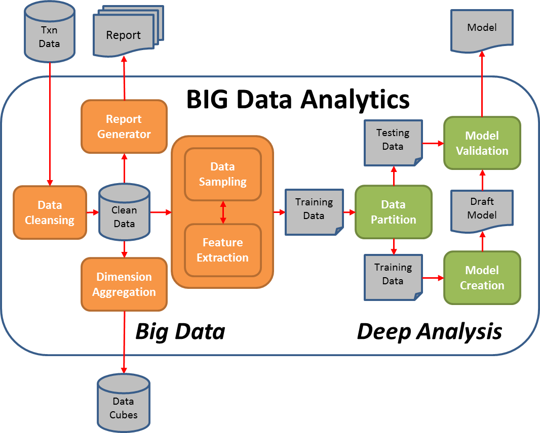
Optimization is usually integrated with predictive analytics, which is another important part of data analytics.  For an overview of predictive analytics, here is my previous blog about it.

The overall processing can be depicted as follows:

In this diagram, we use machine learning to train a predictive model in batch mode.  Once the predictive model is available, observation data is fed into it at real time and a set of output variables is predicted.  Such output variable will be fed into the optimization model as the environment parameters (e.g. return of each stock, covariance ... etc.) from which a set of optimal decision variable is recommended.

MapReduce: Detecting Cycles in Network Graph

I recently received an email from an audience of my blog on Map/Reduce algorithm design regarding how to detect whether a graph is acyclic using Map/Reduce.  I think this is an interesting problem and can imagine there can be wide range of application to it.

Although I haven't solved this exact problem in the past, I'd like to sketch out my thoughts on a straightforward approach, which may not be highly optimized.  My goal is to invite other audience who has solved this problem to share their tricks.

To define the problem:  Given a simple directed graph, we want to tell whether it contains any cycles.

Lets say the graph is represented in incidence edge format where each line represent an edge from one node to another node.  The graph can be split into multiple files.

node1, node2
node4, node7
node7, node1
....

Here is a general description of the algorithm.

We'll maintain two types of graph data.

1. A set of link files where each line represent an edge in the graph.  This file will be static.
2. A set of path files where each line represent a path from one node to another node.  This file will be updated in each round of map/reduce.

The general idea is to grow the path file until either the path cannot grow further, or the path contain a cycle, we'll use two global flags to keep track of that: "change" flag to keep track of whether new path is discovered, and "cycle" flag to keep track whether a cycle is detected.

The main driver program will create the initial path file by copying the link file.  And it will set the initial flag condition:  Set cycle and change flag to true.  In each round, the driver will

• Check if the cycle is still false and change is true, exit if this is not the case
• Otherwise, it will clear the change flag and invoke the map/reduce

Within each round, the map function will do the following

• Emit the tuple [key=toNode, value=fromNode] if it is a path
• Emit the tuple [key=fromNode, value=toNode] if it is a link

This ensure a path and all extended link reaches the same reducer, which will do the following

• Check to see if the beginning point of the path is the same as the endpoint of the link.  If so, it detects a cycle and mark the cycle flag to be true.
• Otherwise, it compute the product of every path to every link, and form the new path which effectively extend the length by one.

The following diagram illustrates the algorithm ...

Detecting Communities in Social Graph

In analyzing social network, one common problem is how to detecting communities, such as groups of people who knows or interacting frequently with each other.  Community is a subgraph of a graph where the connectivity are unusually dense.

In this blog, I will enumerate some common algorithms on finding communities.

First of all, community detection can be think of graph partitioning problem.  In this case, a single node will belong to no more than one community.  In other words, community does not overlap with each other.

High Betweenness Edge Removal

The intuition is that members within a community are densely connected and have many paths to reach each other.  On the other hand, nodes from different communities requires inter-community links to reach each other, and these inter-community links tends to have high betweenness score.

Therefore, by removing these high-betweenness links, the graph will be segregated into communities.

Algorithm:

1. For each edge, compute the edge-betweenness score
2. Remove the edge with the highest betweenness score
3. Until there are enough segregation

However, while this method achieve good result, it is very slow and not work effectively when there are more than couple thousand nodes with dense edges.

Hierarchical Clustering

This is a very general approach of detecting communities.  Some measure of distance (or similarities) is defined and computed between every pair of nodes first.  Then classical hierarchical cluster technique can be applied.  The distance should be chosen such that it is small between members within a community and big between members of different community.

Random Walk

Random walk can be used to compute the distance between every pair of nodes node-B and node-C.  Lets focus on undirected graph for now.  A random walker starts at node-B, throw a dice and has beta probability that it randomly pick a neighbor to visit based on the weight of links, and with 1 - beta probability that it will teleport back to the original node-v.  At an infinite number of steps, the probability distribution of landing on node-w will be high if node-B and node-C belongs to the same community.  The intuition here is that the random walker tends to be trapped within the community so all nodes that has high probability distribution tends to be within the same community as node-B (where the random walker is started).

Notice that the pick of beta is important.  If it is too big (close to 1), then the probability after converging is independent of the starting node (ie: the probability distribution only reflect the centrality of each node but not the community of the starting node).  If beta is too small (close to zero), then the walker will die down too quick before it fully explore the community's connectivity.

There is an analytical solution to this problem.

Lets M be the transition matrix before every pair of nodes. V represents the probability distribution of where the random walkers is.

 The "distance" between node-B and every other nodes is the eigenvector of M.  We can repeat the same to find out distance of all pairs of nodes, and then feed the result to a hierarchical clustering algorithm.

Label Propagation

The basic idea is that nodes observe its neighbors and set its own label to be the majority of its neighbors.

1. Nodes are initially assigned with a unique label.
2. In each round, each node examine the label of all its neighbors are set its own label to be the majority of its neighbors, when there is a tie, the winner is picked randomly.
3. Until there is no more change of label assignments

Modularity Optimization

Within a community, the probability of 2 nodes having a link should be higher than if the link is just formed randomly within the whole graph.

probability of random link = deg(node-B) * deg(node-C) / (N * (N-1))
The actual link = Adjacency matrix[B, C]

Define com(B) to be community of node-B, com(C) to be community of node-C

So a utility function "Modularity" is created as follows ...
sum_over_v_w((actual - random) * delta(com(B), com(C)))


Now we examine communities that can be overlapping.  ie: A single node can belong to more than one community.

Finding Clique

Simple community detection usually starts with cliques.  Clique is a subgraph whether every node is connected to any other node.  In a K-Clique, there are K nodes and K^2 links between them.

However, communities has a looser definition, we don't require everyone to know every other people within the community, but we need them to know "enough" (maybe a certain percentage) of other people in the community.  K-core is more relaxed definition, it requires the nodes of the K-core to have connectivity to at least K other members.  There are some less popular relaxation, K-Clan requires every node to connect with every other members within K steps (path length less than K).  K-plex requires the node to connect to (N - K) members in the node where N total number of members within the K-plex.

The community is defined as the found K-core, or K-clan, or K-plex.

K-Clique Percolation

Another popular way of finding community is by rolling across adjacent K-Clique.  Two K-Clique is adjacent if they share K-1 nodes.  K is a parameter that we need to pick based on how dense we expect the community should have.

The algorithm is illustrated in following diagram.

K-Clique percolation is a popular way to identify communities which can potentially be overlapping with each other.

Machine Learning in Gradient Descent

In Machine Learning, gradient descent is a very popular learning mechanism that is based on a greedy, hill-climbing approach.

Gradient Descent

The basic idea of Gradient Descent is to use a feedback loop to adjust the model based on the error it observes (between its predicted output and the actual output).  The adjustment (notice that there are multiple model parameters and therefore should be considered as a vector) is pointing to a direction where the error is decreasing in the steepest sense (hence the term "gradient").

Notice that we intentionally leave the following items vaguely defined so this approach can be applicable in a wide range of machine learning scenarios.

• The Model
• The loss function
• The learning rate

Gradient Descent is very popular method because of the following reasons ...

• Intuitive and easy to understand
• Easy to run in parallel processing architecture
• Easy to run incrementally with additional data

On the other hand, the greedy approach in Gradient Descent can be trapped in local optimum.  This can be mitigated by choosing a convex LOSS function (which has a single optimum), or multiple starting points can be picked randomly (in the case, we hope the best local optimum is close to the global optimum).

Batch vs Online Learning

While some other Machine Learning model (e.g. decision tree) requires a batch of data points before the learning can start, Gradient Descent is able to learn each data point independently and hence can support both batch learning and online learning easily.  The difference lies in how the training data is fed into the model and how the loss function computes its error.

In batch learning, all training will be fed to the model, who estimates the output for all data points.  Error will then be summed to compute the loss and then update the model.  Model in this case will be updated after predicting the whole batch of data points.

In online learning mode (also called stochastic gradient descent), data is fed to the model one at a time while the adjustment of the model is immediately made after evaluating the error of this single data point.  Notice that the final result of incremental learning can be different from batch learning, but it can be proved that the difference is bound and inversely proportional to the square root of the number of data points.

The learning rate can be adjusted as well to achieve a better stability in convergence.  In general, the learning rate is higher initially and decrease over the iteration of training (in batch learning it decreases in next round, in online learning it decreases at every data point).  This is quite intuitive as you paid less attention to the error as you have learn more and more.  Because of that online learning is sensitive to the arrival order of data.

One way to adjust the learning rate is to have a constant divide by the square root of N (where N is the number of data point seen so far).

 ɳ = ɳ_initial / (t ^ 0.5).

By using different decay factor, we can control how much attention we should pay for the late coming data.  In online learning, as data comes in time of occurrence, we can play around with this decay factor to guide how much attention the learning mechanism should be paying to latest arrival data.  Online learning automatically adapt to change of trends over time.

Most real world machine learning scenario relies on stationality of the model.  By the way, learning is about "learning from past experience".  If the environment changes too rapidly that the past experience is invalid, there is little value to learn.  Because of this reason, most machine learning project are satisfied by using batch learning (daily or weekly) and the demand of online learning is not very high.  A very common batch learning model is described in my previous blog here.

Parallel Learning

Because of no dependency in data processing, Gradient Descent is very easy to put into a parallel processing environment such as Map/Reduce.  Here we illustrate how to parallelize the execution of batch learning.

Notice that there are multiple rounds of Map/Reduce until the model converges.  On the other hand, online learning is not possible for Hadoop Map/Reduce which doesn't support real-time at this moment.

In summary, gradient descent is a very powerful approach of machine learning and works well in a wide spectrum of scenarios.

Location Sensitive Hashing in Map Reduce

Inspired by Dr. Gautam Shroff who teaches the class: Web Intelligence and Big data in coursera.org, there are many scenarios where we want to compute similarity between large amount of items (e.g. photos, products, persons, resumes ... etc).  I want to add another algorithm to my Map/Reduce algorithm catalog.

For the background of Map/Reduce implementation on Hadoop.  I have a previous post that covers the details.

Large Scale Similarity Computation

Lets say there are N items (N is billions) and we want to find all those that are similar to each other.  (similarity is defined by a distance function).  The goal is to output a similarity matrix.  (Notice that this matrix is very sparse and most of the cells are infinite)

One naive way is to compute the similarity of each possible pairs of items, hence an O(N^2) problem which is huge.  Can we reduce the order of complexity ?

Location Sensitive Hashing

First idea: Find a hashing function such that similar items (say distance is less than some predefined threshold) will be hashed to the same bucket.

Lets say if we pick the hash function such that Probability(H(a) == H(b)) is proportional to similarity between a and b.  And then we only perform detail comparison on items that falls into the same bucket.

Here is some R code that plots the relationship between similarity and the chance of performing a detail comparison.

x <- seq(0, 1, 0.01)
y <- x
plot(x, y, xlab="similarity", ylab="prob of detail compare")

Lets say we are interested in comparing all pairs of items whose similarity is above 0.3, we have a problem here because we have probability 0.7 = 1 - 0.3 of missing them (as they are not landing on the same bucket).  We want a mechanism that is highly selective; probability of performing a detail comparison should be close to one when similarity is above 0.3 and close to zero when similarity is below 0.3.

Second idea: Lets use 100 hash functions and 2 items that has 30 or more matches of such hash functions will be selected for detail comparison.

Here is some R code that plots the relationship between similarity and the chance of performing a detail comparison.

# Probability of having more than "threshold" matches out 
# of "no_of_hash" with a range of varying similarities

prob_select <- function(threshold, similarity, no_of_hash) {
  sum <- rep(0, length(similarity))
  for (k in 0:floor(no_of_hash * threshold)) {
    sum <- sum + dbinom(k, no_of_hash, similarity)
  }
  return(1 - sum)
}

x <- seq(0, 1, 0.01)
y <- prob_select(0.3, x, 100)
plot(x, y, main="black: 100 hashes, Red: 1000 hashes", 
xlab="similarity", ylab="prob of detail compare")
lines(x, y)
y <- prob_select(0.3, x, 1000)
lines(x, y, col="red")

The graph looks much better this time, the chance of being selected for detail comparison jumps from zero to one sharply when the similarity crosses 0.3

To compare the items that are similar, we first compute 100 hashes (based on 100 different hash functions) for each item and output all combination 30 hashes as a key.  Then we perform pairwise comparison for all items that has same key.

But look at the combination of 30 out of 100, it is 100!/(30! * 70!) = 2.93 * 10^25, which is impractically huge.  Even the graph is a nice, we cannot use this mechanism in practice.

Third idea: Lets use 100 hash function and break them into b groups of r each (ie: b*r = 100).  Further let assume b = 20, and r = 5.  In other words, we have 20 groups and Group1 has hash1 to hash5, Group2 has hash6 to hash10 ... etc.  Now, we call itemA's group1 matches itemB's group1 if all their hash1 to hash5 are equal to each other.  Now, we'll perform a detail comparison of itemA and itemB if any of the groups are equal to each other.

Probability of being selected is  1 - (1-s^r)^b

The idea can be visualized as follows

Notice that in this model, finding r and b based on s is a bit trial and error.  Here we try 20 by 5, 33 by 3, 10 by 10.

prob_select2 <- function(similarity, row_per_grp, no_of_grp) {
  return(1 - (1 - similarity^row_per_grp)^no_of_grp)
}

x <- seq(0, 1, 0.01)
y <- prob_select2(x, 5, 20)

plot(x, y, 
main="black:20 by 5, red:10 by 10, blue:33 by 3", 
xlab="similarity", ylab="prob of detail compare")

lines(x, y)
y <- prob_select2(x, 10, 10)
lines(x, y, col="red")
y <- prob_select2(x, 3, 33)
lines(x, y, col="blue")

From the graph, we see the blue curve fits better to select the similarity at 0.3.  So lets use 33 by 3.

Notice that the ideal graph should be a step function where probability jumps from 0 to 1 when similarity cross over the similarity threshold that we are interested to capture (ie: we want to put all pairs whose similarity bigger than this threshold to be in a same bucket and all pairs whose similarity less that this threshold to be in a different bucket).  Unfortunately, our curve is a S-curve, not a step function.  This means there will be false positive and false negative.  False position lies on the left side of the similarity threshold where we have a small chance to put them into the same bucket, which will cost up some extra work to compare them later and throw them away.  On the other hand, false negative lies on the right side where we have a small chance of putting items that are very similar into different buckets and not considering them in the detail comparison.  Depends on whether we need to catch all the similar items above the threshold, we may need shift the S curve left or right by tuning the r and b parameters. 

To perform the detail comparison, we can use a parallel Map/Reduce implementation

Map Reduce Implementation

Here we have two round of Map/Reduce.  In the first round, map function will compute all the groupKeys for each item and emit the groupKey with the item.  All the items that has the groupKey matches will land on the same reducer, which creates all the possible pairs of items (these are candidates for pairwise comparison).

However, we don't want to perform the detail comparison in the first round as there may be many duplicates for item pairs that matches more than one group.  Therefore we want to perform another round of Map/reduce to remove the duplicates.

The first round proceeds as follows ...

After that, the second round proceeds as follows ...

By combining Location Sensitive Hashing and Map/Reduce,  we can perform large scale similarity calculation in an effective manner.

BIG Data Analytics Pipeline

"Big Data Analytics" has recently been one of the hottest buzzwords.  It is a combination of "Big Data" and "Deep Analysis".  The former is a phenomenon of Web2.0 where a lot of transaction and user activity data has been collected which can be mined for extracting useful information.  The later is about using advanced mathematical/statistical technique to build models from the data.  In reality I've found these two areas are quite different and disjoint and people working in each area have a pretty different background.

Big Data Camp

People working in this camp typically come from Hadoop, PIG/Hive background.  They usually have implemented some domain-specific logic to process large amount of raw data.  Often the logic is relatively straight-forward based on domain-specific business rules.

From my personal experience, most of the people working in big data come from a computer science and distributed parallel processing system background but not from the statistical or mathematical discipline.

Deep Analysis Camp

On the other hand, people working in this camp usually come from statistical and mathematical background which the first thing being taught is how to use sampling to understand a large population's characteristic.  Notice the magic of "sampling" is that the accuracy of estimating the large population depends only in the size of sample but not the actual size of the population.  In their world, there is never a need to process all the data in the population in the first place.  Therefore, Big Data Analytics is unnecessary under this philosophy.

Typical Data Processing Pipeline

Learning from my previous projects, I observe most data processing pipeline fall into the following pattern.

In this model, data is created from the OLTP (On Line Transaction Processing) system, flowing into the BIG Data Analytics system which produced various output; including data mart/cubes for OLAP (On Line Analytic Processing), reports for the consumption of business executives, and predictive models that feedback decision support for OLTP.

Big Data + Deep Analysis

The BIG data analytics box is usually done in a batch fashion (e.g. once a day), usually we see big data processing and deep data analysis happens at different stages of this batch process.

The big data processing part (colored in orange) is usually done using Hadoop/PIG/Hive technology with classical ETL logic implementation.  By leveraging the Map/Reduce model that Hadoop provides, we can linearly scale up the processing by adding more machines into the Hadoop cluster.  Drawing cloud computing resources (e.g. Amazon EMR) is a very common approach to perform this kind of tasks.

The deep analysis part (colored in green) is usually done in R, SPSS, SAS using a much smaller amount of carefully sampled data that fits into a single machine's capacity (usually less than couple hundred thousands data records).  The deep analysis part usually involve data visualization, data preparation, model learning (e.g. Linear regression and regularization, K-nearest-neighbour/Support vector machine/Bayesian network/Neural network, Decision Tree and Ensemble methods), model evaluation.  For those who are interested, please read up my earlier posts on these topics.

Implementation Architecture

There are many possible ways to implement the data pipeline described above.  Here is one common implementation that works well in many projects.

In this architecture, "Flume" is used to move data from OLTP system to Hadoop File System HDFS.  A workflow scheduler (typically a cron-tab entry calling a script) will periodically run to process the data using Map/Reduce.  The data has two portions:  a) Raw transaction data from HDFS  b) Previous model hosted in some NOSQL server.  Finally the "reducer" will update the previous model which will be available to the OLTP system.

For most the big data analytic projects that I got involved, the above architecture works pretty well.  I believe projects requiring real-time feedback loop may see some limitation in this architecture.  Real-time big data analytics is an interesting topic which I am planning to discuss in future posts.

Measuring similarity and distance function

Measuring similarity or distance between two data points is very fundamental to many Machine Learning algorithms such as K-Nearest-Neighbor, Clustering ... etc.  Depends on the nature of the data point, various measurement can be used.

 

Distance between numeric data points

When the dimension of data point is numeric, the general form is called Minkowski distance

( (x₁ - x₂)^p + (y₁ - y₂)^p )^1/p

When p = 2, this is equivalent to Euclidean distance.  When p = 1, this is equivalent to Manhattan distance.

This measure is independent of the underlying data distribution.  But what if the value along the x-dimension is much bigger than that from the y-dimension.  So we need to bring all of them into the same scale first.  A common way is to perform a z-transform where each data point first subtract the mean value, and then divide the standard deviation.

(x₁, y₁) becomes ( (x₁ – μ_x)/σ_x , (y₁ – μ_y)/σ_y )

This measure, although taking into consideration of the distribution of each dimension, it assumes the dimension are independent of each other.  But what if x-dimension and y-dimension has some correlation.  To consider correlation between different dimensions, we use ...

Mahalanobis distance = (v ₁^→ -  v ₂^→)^T.CovMatrix.(v ₁^→ -  v ₂^→)  where v ₁^→  = (x₁, y₁)

If we care about the direction of the data rather than the magnitude, then cosine distance is a common approach.  It computes the dot product of the two data points divided by the product of their magnitude.  Cosine distance, together with term/document matrix, is commonly used to measure the similarity between documents.

 

Distance between categorical data points

Since there is no ordering between categorical value, we can only measure whether the categorical value is the same or not.  Basically we are measuring the degree of overlapping of attribute values.  Hamming distance can be used to measure how many attributes need to changed in order to match each other.  We can calculate the ratio to determine how similar (or difference) between two data points using simple matching coefficient:
noOfMatchAttributes / noOfAttributes

However, when the data point contains asymmetric binary data attributes, equality of certain value doesn't mean anything.  For example, lets say the data point represents a user with attributes represent each movie.  The data point contains a high dimensional binary value representing whether the user has seen the movie.  (1 represent yes and 0 represent no).  Given that most users only see a very small portion of all movies, if both user hasn't seen a particular movie (both value is zero), it doesn't indicate any similarity between the user.  On the other hand, if both user saw the same movie (both value is one), it implies a lot of similarity between the user.  In this case, equality of one should carry a much higher weight than equality of zero.  This lead to Jaccard similarity :
noOfOnesInBoth / (noOfOnesInA + noOfOnesInB - noOfOnesInAandB)

Besides matching or not, if category is structured as a Tree hierarchy, then the distance of two category can be quantified by path length of their common parent.  For example, "/product/spot/ballgame/basketball" is closer to "/product/spot/ballgame/soccer/shoes" than "/product/luxury/handbags" because the common parent has a longer path.

 

Similarity between instances containing mixed types of attributes

When the data point contain a mixed of attributes, we can calculate the similarity of each attribute (or group the attributes of the same type), and then combine them together using some weighted average.

But we have to be careful when treating asymmetric attributes where its presence doesn't mean anything.

combined_similarity(x, y) = Σ_{over_k}[w_k * δ_k * similarity(x_k, y_k)] / Σ_{over_k}(δ_k)

where Σ_{over_k}(w_k) = 1

Distance between sequence (String, TimeSeries)

In case each attribute represent an element of a sequence, we need a different way to measure the distance.  For example, lets say each data point is a string (which contains a sequence of characters), then edit distance is a common measurement.  Basically, edit distance is how many "modifications" (which can be insert, modify, delete) is needed to change stringA into stringB.  This is usually calculated by using dynamic programming technique.

Time Series is another example of sequence data.  Similar to the concept of edit distance, Dynamic Time Warp is about distorting the time dimension by adding more data points in both time series such that their square error between corresponding pairs is minimized.  Where to add these data points are solved using a similar dynamic programming technique.  Here is a very good paper that describe the details.

 

 Distance between nodes in a network

In a homogenous undirected graph (nodes are of the same type), distance between nodes can be measured by the shortest path.

In a bi-partite graph, there are two types of nodes in which each node only connects to the other type.  (e.g. People joining Communities).  Similarity between nodes (of same type) can be measured by analyzing how similar their connected communities are.

SimRank is an iterative algorithm that compute the similarity of each type of nodes by summing the similarity between all pairs of other type of nodes that it has connected, while other type of nodes' similarity is computed in the same way.

We can also use a probabilistic approach such as RandomWalk to determine the similarity.  Each people node will pass a token (label with the people's name) along a randomly picked community node which it is connected to (weighted by the strength of connectivity).  Each community node will propagated back the received token back to a randomly picked people.  Now the people who received the propagated token may drop the token (with a chance beta) or propagated to a randomly chosen community again.  This process continues under all the tokens are die out (since they have a chance of being dropped).  After that, we obtain the trace Matrix and compute the similarity based on the dot product of the tokens it receives.

 

Distance between population distribution

Instead of measuring distance between individual data points, we can also compare a collection of data points (ie: population) and measure the distance between them.  In fact, one important part of statistics is to measure the distance between two groups of samples and see if the "difference" is significant enough to conclude they are from different populations.

Lets say the population contains members that belongs to different categories and we want to measure if population A and population B have same or different proportions of members across these categories, then we can use Chi-Square or KL-Divergence to measure their distance.

In case every member of the population has two different numeric attributes (e.g. weight and height), and we want to infer one attribute from the other if they are correlated, correlation coefficient is a measure that quantify their degree of correlation; whether these two attributes are moving along the same direction (heavier people are taller), different direction (heavier people are shorter), or independent.  The correlation coefficient ranges from -1 (negatively correlated) to 0 (no correlation) to 1 (positively correlated).

If the two attributes are categorical (rather than numeric), then mutual information is a common way to measure their dependencies and give a good sense of whether knowing the value of one attribute can help inferring the other attribute.

Now if there are two judges who rank a collection of items and we are interested in the degree of agreement of their ranking order.  We can use Spearman's rank coefficient to measure their degree of consensus in the ranking order.